Inspecting your data in tables#
This tutorial shows how to leverage xarray and pandas to easily transform xsnowDatasets into tidy, tabular views that you can scan like a spreadsheet.
In particular,
Select an individual profile and view it as a
pandas.DataFrameKeep or drop length-1 dimensions with
.squeeze()when flattening arraysInspect data points of your interest by applying a mask with
.where()Export summaries to pandas
Series/DataFrameor NumPy arrays
Handy helpers
Object |
Method |
Description |
|---|---|---|
Dataset / DataArray |
Squeeze out all dimensions of length 1. |
|
Dataset / DataArray |
Convert this dataset or data array into a tidy |
|
DataArray |
Convert this array into a pandas object ( |
|
DataArray |
Coerce to a NumPy array. |
import xsnow
import pandas as pd

xs = xsnow.single_profile_timeseries()
print(xs.sizes)
[i] xsnow.xsnow_io: Analyzing file sizes for 2 files...
[i] xsnow.xsnow_io: File size range: 4592.3KB - 4816.0KB
[i] xsnow.xsnow_io: Scanning 2 largest files to determine max layer count...
[i] xsnow.xsnow_io: ✅ Smart max_layers determination complete:
[i] xsnow.xsnow_io: - Checked: 2 file sizes
[i] xsnow.xsnow_io: - Scanned: 2 largest files
[i] xsnow.xsnow_io: - Max layers found: 59
[i] xsnow.xsnow_io: - Using max_layers: 59 (exact - scanned all files)
[i] xsnow.xsnow_io: - Time elapsed: 0.04 seconds
[i] xsnow.xsnow_io: Loading 2 datasets eagerly with 1 workers...
[i] xsnow.utils: Slope coordinate 'inclination' varies by location. Preserving (location, slope) dimensions as allow_per_location=True.
[i] xsnow.utils: Slope coordinate 'azimuth' varies by location. Preserving (location, slope) dimensions as allow_per_location=True.
Frozen({'location': 1, 'time': 381, 'slope': 1, 'realization': 1, 'layer': 59})
1. Inspect a single profile as a table#
Select one timestamp/slope/realization and turn the subset of variables into a DataFrame for a spreadsheet-like view.
profile = xs.isel(time=-1, slope=0, realization=[0])
profile.sizes
Frozen({'location': 1, 'realization': 1, 'layer': 59})
You see that sel and isel squeeze length-1 dimensions by default when given as scalars (e.g., time and slope in the example above) unless they are given as lists (e.g., realization).
profile[['height', 'sk38', 'density']].to_dataframe()
| height | sk38 | density | altitude | azimuth | inclination | latitude | longitude | time | slope | z | |||
|---|---|---|---|---|---|---|---|---|---|---|---|---|---|
| location | realization | layer | |||||||||||
| Kasererwinkl_C6 | 0 | 0 | 1.750000 | 6.00 | 520.200012 | 1681.0 | 270 | 16 | 47.10183 | 11.61714 | 2024-02-02 12:00:00 | 0 | -101.459999 |
| 1 | 3.500000 | 3.50 | 520.000000 | 1681.0 | 270 | 16 | 47.10183 | 11.61714 | 2024-02-02 12:00:00 | 0 | -99.709999 | ||
| 2 | 5.250000 | 3.53 | 519.500000 | 1681.0 | 270 | 16 | 47.10183 | 11.61714 | 2024-02-02 12:00:00 | 0 | -97.959999 | ||
| 3 | 7.000000 | 2.51 | 518.900024 | 1681.0 | 270 | 16 | 47.10183 | 11.61714 | 2024-02-02 12:00:00 | 0 | -96.209999 | ||
| 4 | 8.850000 | 2.04 | 347.700012 | 1681.0 | 270 | 16 | 47.10183 | 11.61714 | 2024-02-02 12:00:00 | 0 | -94.360001 | ||
| 5 | 10.720000 | 2.06 | 347.100006 | 1681.0 | 270 | 16 | 47.10183 | 11.61714 | 2024-02-02 12:00:00 | 0 | -92.489998 | ||
| 6 | 12.580000 | 2.08 | 346.600006 | 1681.0 | 270 | 16 | 47.10183 | 11.61714 | 2024-02-02 12:00:00 | 0 | -90.629997 | ||
| 7 | 14.460000 | 2.10 | 346.000000 | 1681.0 | 270 | 16 | 47.10183 | 11.61714 | 2024-02-02 12:00:00 | 0 | -88.750000 | ||
| 8 | 16.330000 | 2.12 | 345.399994 | 1681.0 | 270 | 16 | 47.10183 | 11.61714 | 2024-02-02 12:00:00 | 0 | -86.879997 | ||
| 9 | 18.209999 | 2.14 | 344.899994 | 1681.0 | 270 | 16 | 47.10183 | 11.61714 | 2024-02-02 12:00:00 | 0 | -85.000000 | ||
| 10 | 20.090000 | 2.16 | 344.399994 | 1681.0 | 270 | 16 | 47.10183 | 11.61714 | 2024-02-02 12:00:00 | 0 | -83.119995 | ||
| 11 | 21.980000 | 2.19 | 343.899994 | 1681.0 | 270 | 16 | 47.10183 | 11.61714 | 2024-02-02 12:00:00 | 0 | -81.229996 | ||
| 12 | 23.860001 | 2.21 | 343.500000 | 1681.0 | 270 | 16 | 47.10183 | 11.61714 | 2024-02-02 12:00:00 | 0 | -79.349998 | ||
| 13 | 25.750000 | 2.23 | 343.100006 | 1681.0 | 270 | 16 | 47.10183 | 11.61714 | 2024-02-02 12:00:00 | 0 | -77.459999 | ||
| 14 | 27.639999 | 2.25 | 342.799988 | 1681.0 | 270 | 16 | 47.10183 | 11.61714 | 2024-02-02 12:00:00 | 0 | -75.570000 | ||
| 15 | 29.530001 | 2.10 | 342.500000 | 1681.0 | 270 | 16 | 47.10183 | 11.61714 | 2024-02-02 12:00:00 | 0 | -73.680000 | ||
| 16 | 31.240000 | 2.15 | 316.000000 | 1681.0 | 270 | 16 | 47.10183 | 11.61714 | 2024-02-02 12:00:00 | 0 | -71.970001 | ||
| 17 | 32.950001 | 2.17 | 316.100006 | 1681.0 | 270 | 16 | 47.10183 | 11.61714 | 2024-02-02 12:00:00 | 0 | -70.259995 | ||
| 18 | 34.450001 | 2.39 | 520.200012 | 1681.0 | 270 | 16 | 47.10183 | 11.61714 | 2024-02-02 12:00:00 | 0 | -68.759995 | ||
| 19 | 36.450001 | 2.06 | 347.000000 | 1681.0 | 270 | 16 | 47.10183 | 11.61714 | 2024-02-02 12:00:00 | 0 | -66.759995 | ||
| 20 | 38.439999 | 2.08 | 347.500000 | 1681.0 | 270 | 16 | 47.10183 | 11.61714 | 2024-02-02 12:00:00 | 0 | -64.770004 | ||
| 21 | 40.439999 | 2.10 | 347.700012 | 1681.0 | 270 | 16 | 47.10183 | 11.61714 | 2024-02-02 12:00:00 | 0 | -62.770000 | ||
| 22 | 42.439999 | 2.11 | 347.899994 | 1681.0 | 270 | 16 | 47.10183 | 11.61714 | 2024-02-02 12:00:00 | 0 | -60.770000 | ||
| 23 | 44.439999 | 2.11 | 348.700012 | 1681.0 | 270 | 16 | 47.10183 | 11.61714 | 2024-02-02 12:00:00 | 0 | -58.770000 | ||
| 24 | 46.439999 | 2.81 | 520.900024 | 1681.0 | 270 | 16 | 47.10183 | 11.61714 | 2024-02-02 12:00:00 | 0 | -56.770000 | ||
| 25 | 48.439999 | 1.16 | 519.099976 | 1681.0 | 270 | 16 | 47.10183 | 11.61714 | 2024-02-02 12:00:00 | 0 | -54.770000 | ||
| 26 | 50.419998 | 1.44 | 272.500000 | 1681.0 | 270 | 16 | 47.10183 | 11.61714 | 2024-02-02 12:00:00 | 0 | -52.790001 | ||
| 27 | 52.380001 | 1.47 | 278.200012 | 1681.0 | 270 | 16 | 47.10183 | 11.61714 | 2024-02-02 12:00:00 | 0 | -50.829998 | ||
| 28 | 54.320000 | 1.45 | 279.600006 | 1681.0 | 270 | 16 | 47.10183 | 11.61714 | 2024-02-02 12:00:00 | 0 | -48.889999 | ||
| 29 | 56.270000 | 1.41 | 279.399994 | 1681.0 | 270 | 16 | 47.10183 | 11.61714 | 2024-02-02 12:00:00 | 0 | -46.939999 | ||
| 30 | 58.220001 | 0.75 | 279.000000 | 1681.0 | 270 | 16 | 47.10183 | 11.61714 | 2024-02-02 12:00:00 | 0 | -44.989998 | ||
| 31 | 59.779999 | 0.93 | 210.100006 | 1681.0 | 270 | 16 | 47.10183 | 11.61714 | 2024-02-02 12:00:00 | 0 | -43.430000 | ||
| 32 | 61.349998 | 0.91 | 209.199997 | 1681.0 | 270 | 16 | 47.10183 | 11.61714 | 2024-02-02 12:00:00 | 0 | -41.860001 | ||
| 33 | 62.919998 | 0.89 | 208.199997 | 1681.0 | 270 | 16 | 47.10183 | 11.61714 | 2024-02-02 12:00:00 | 0 | -40.290001 | ||
| 34 | 64.510002 | 0.86 | 207.100006 | 1681.0 | 270 | 16 | 47.10183 | 11.61714 | 2024-02-02 12:00:00 | 0 | -38.699997 | ||
| 35 | 66.099998 | 0.83 | 206.100006 | 1681.0 | 270 | 16 | 47.10183 | 11.61714 | 2024-02-02 12:00:00 | 0 | -37.110001 | ||
| 36 | 67.699997 | 0.79 | 204.899994 | 1681.0 | 270 | 16 | 47.10183 | 11.61714 | 2024-02-02 12:00:00 | 0 | -35.510002 | ||
| 37 | 69.309998 | 0.77 | 203.000000 | 1681.0 | 270 | 16 | 47.10183 | 11.61714 | 2024-02-02 12:00:00 | 0 | -33.900002 | ||
| 38 | 70.919998 | 0.73 | 202.800003 | 1681.0 | 270 | 16 | 47.10183 | 11.61714 | 2024-02-02 12:00:00 | 0 | -32.290001 | ||
| 39 | 71.739998 | 1.74 | 61.000000 | 1681.0 | 270 | 16 | 47.10183 | 11.61714 | 2024-02-02 12:00:00 | 0 | -31.470001 | ||
| 40 | 72.440002 | 0.68 | 202.399994 | 1681.0 | 270 | 16 | 47.10183 | 11.61714 | 2024-02-02 12:00:00 | 0 | -30.769997 | ||
| 41 | 73.500000 | 0.38 | 237.600006 | 1681.0 | 270 | 16 | 47.10183 | 11.61714 | 2024-02-02 12:00:00 | 0 | -29.709999 | ||
| 42 | 75.599998 | 0.58 | 178.100006 | 1681.0 | 270 | 16 | 47.10183 | 11.61714 | 2024-02-02 12:00:00 | 0 | -27.610001 | ||
| 43 | 76.730003 | 0.52 | 251.899994 | 1681.0 | 270 | 16 | 47.10183 | 11.61714 | 2024-02-02 12:00:00 | 0 | -26.479996 | ||
| 44 | 77.889999 | 0.37 | 282.700012 | 1681.0 | 270 | 16 | 47.10183 | 11.61714 | 2024-02-02 12:00:00 | 0 | -25.320000 | ||
| 45 | 79.019997 | 0.33 | 268.000000 | 1681.0 | 270 | 16 | 47.10183 | 11.61714 | 2024-02-02 12:00:00 | 0 | -24.190002 | ||
| 46 | 79.540001 | 0.21 | 260.799988 | 1681.0 | 270 | 16 | 47.10183 | 11.61714 | 2024-02-02 12:00:00 | 0 | -23.669998 | ||
| 47 | 81.599998 | 0.34 | 236.300003 | 1681.0 | 270 | 16 | 47.10183 | 11.61714 | 2024-02-02 12:00:00 | 0 | -21.610001 | ||
| 48 | 83.650002 | 0.09 | 236.600006 | 1681.0 | 270 | 16 | 47.10183 | 11.61714 | 2024-02-02 12:00:00 | 0 | -19.559998 | ||
| 49 | 85.980003 | 6.00 | 226.399994 | 1681.0 | 270 | 16 | 47.10183 | 11.61714 | 2024-02-02 12:00:00 | 0 | -17.229996 | ||
| 50 | 87.150002 | 6.00 | 216.000000 | 1681.0 | 270 | 16 | 47.10183 | 11.61714 | 2024-02-02 12:00:00 | 0 | -16.059998 | ||
| 51 | 89.440002 | 6.00 | 218.699997 | 1681.0 | 270 | 16 | 47.10183 | 11.61714 | 2024-02-02 12:00:00 | 0 | -13.769997 | ||
| 52 | 90.540001 | 6.00 | 220.600006 | 1681.0 | 270 | 16 | 47.10183 | 11.61714 | 2024-02-02 12:00:00 | 0 | -12.669998 | ||
| 53 | 93.330002 | 6.00 | 177.600006 | 1681.0 | 270 | 16 | 47.10183 | 11.61714 | 2024-02-02 12:00:00 | 0 | -9.879997 | ||
| 54 | 95.239998 | 6.00 | 130.800003 | 1681.0 | 270 | 16 | 47.10183 | 11.61714 | 2024-02-02 12:00:00 | 0 | -7.970001 | ||
| 55 | 96.980003 | 6.00 | 149.399994 | 1681.0 | 270 | 16 | 47.10183 | 11.61714 | 2024-02-02 12:00:00 | 0 | -6.229996 | ||
| 56 | 99.010002 | 6.00 | 137.399994 | 1681.0 | 270 | 16 | 47.10183 | 11.61714 | 2024-02-02 12:00:00 | 0 | -4.199997 | ||
| 57 | 101.050003 | 6.00 | 127.699997 | 1681.0 | 270 | 16 | 47.10183 | 11.61714 | 2024-02-02 12:00:00 | 0 | -2.159996 | ||
| 58 | 103.209999 | 6.00 | 76.500000 | 1681.0 | 270 | 16 | 47.10183 | 11.61714 | 2024-02-02 12:00:00 | 0 | 0.000000 |
The DataFrame is indexed by the dimensions of the former dataset (unless we squeezed them out as we did for slope/time). It contains the data variables that we requested (['height', 'sk38', 'density']), and it contains all the coordinates (['time', 'slope', 'latitude', 'longitude', 'altitude', 'inclination', 'azimuth', 'z']).
2. Mask values before turning them into tables#
For larger datasets, you often want to keep only layers that pass a condition. Build a simple mask (with where()—see also Subsetting and Filtering), preserve the grid shape, and inspect the remaining rows with pandas.
# Stability index across time and layer
xs2d = xs.squeeze()
print('Before squeeze:', xs.sizes)
print('After squeeze :', xs2d.sizes)
Before squeeze: Frozen({'location': 1, 'time': 381, 'slope': 1, 'realization': 1, 'layer': 59})
After squeeze : Frozen({'time': 381, 'layer': 59})
sk38_masked = xs2d[['sk38', 'rta']].where(xs2d['rta'] > 0.8)
sk38_masked.to_dataframe().dropna()
| sk38 | rta | altitude | azimuth | inclination | latitude | location | longitude | slope | realization | z | ||
|---|---|---|---|---|---|---|---|---|---|---|---|---|
| time | layer | |||||||||||
| 2024-01-17 16:00:00 | 19 | 2.04 | 0.85 | 1681.0 | 270 | 16 | 47.10183 | Kasererwinkl_C6 | 11.61714 | 0 | 0 | -39.989998 |
| 23 | 1.58 | 0.87 | 1681.0 | 270 | 16 | 47.10183 | Kasererwinkl_C6 | 11.61714 | 0 | 0 | -31.989998 | |
| 26 | 0.74 | 1.00 | 1681.0 | 270 | 16 | 47.10183 | Kasererwinkl_C6 | 11.61714 | 0 | 0 | -25.989998 | |
| 2024-01-17 17:00:00 | 19 | 2.04 | 0.85 | 1681.0 | 270 | 16 | 47.10183 | Kasererwinkl_C6 | 11.61714 | 0 | 0 | -39.989998 |
| 23 | 1.58 | 0.87 | 1681.0 | 270 | 16 | 47.10183 | Kasererwinkl_C6 | 11.61714 | 0 | 0 | -31.989998 | |
| ... | ... | ... | ... | ... | ... | ... | ... | ... | ... | ... | ... | ... |
| 2024-02-02 12:00:00 | 36 | 0.79 | 0.81 | 1681.0 | 270 | 16 | 47.10183 | Kasererwinkl_C6 | 11.61714 | 0 | 0 | -35.510002 |
| 37 | 0.77 | 0.81 | 1681.0 | 270 | 16 | 47.10183 | Kasererwinkl_C6 | 11.61714 | 0 | 0 | -33.900002 | |
| 39 | 1.74 | 0.96 | 1681.0 | 270 | 16 | 47.10183 | Kasererwinkl_C6 | 11.61714 | 0 | 0 | -31.470001 | |
| 40 | 0.68 | 0.97 | 1681.0 | 270 | 16 | 47.10183 | Kasererwinkl_C6 | 11.61714 | 0 | 0 | -30.769997 | |
| 42 | 0.58 | 0.89 | 1681.0 | 270 | 16 | 47.10183 | Kasererwinkl_C6 | 11.61714 | 0 | 0 | -27.610001 |
1950 rows × 11 columns
3. Summaries and exports#
After masking, let’s reduce along layer and export to different data structures. Note that you would mostly run computations on the DataArrays, no need to convert them.
Here, we are interested in the minimum SK38 per timestamp:
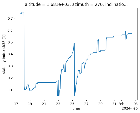
sk38_min = sk38_masked['sk38'].min('layer', skipna=True)
print(sk38_min)
<xarray.DataArray 'sk38' (time: 381)> Size: 2kB
array([0.74, 0.74, 0.74, 0.74, 0.75, 0.75, 0.75, 0.75, 0.75, 0.75, 0.75,
       0.75, 0.13, 0.1 , 0.1 , 0.1 , 0.1 , 0.1 , 0.11, 0.11, 0.11, 0.13,
       0.14, 0.14, 0.14, 0.14, 0.14, 0.14, 0.11, 0.11, 0.11, 0.09, 0.09,
       0.09, 0.09, 0.09, 0.09, 0.09, 0.09, 0.1 , 0.1 , 0.1 , 0.11, 0.11,
       0.11, 0.11, 0.12, 0.12, 0.12, 0.12, 0.12, 0.12, 0.15, 0.15, 0.15,
       0.15, 0.15, 0.15, 0.16, 0.16, 0.16, 0.16, 0.16, 0.16, 0.16, 0.16,
       0.16, 0.16, 0.16, 0.16, 0.16, 0.16, 0.16, 0.16, 0.16, 0.16, 0.16,
       0.16, 0.16, 0.16, 0.16, 0.16, 0.16, 0.16, 0.16, 0.16, 0.16, 0.16,
       0.16, 0.16, 0.16, 0.16, 0.16, 0.16, 0.16, 0.16, 0.16, 0.16, 0.16,
       0.16, 0.16, 0.16, 0.16, 0.16, 0.16, 0.16, 0.16, 0.16, 0.16, 0.16,
       0.16, 0.16, 0.16, 0.16, 0.16, 0.16, 0.16, 0.16, 0.16, 0.16, 0.16,
       0.17, 0.17, 0.17, 0.17, 0.06, 0.05, 0.13, 0.18, 0.05, 0.05, 0.05,
       0.09, 0.09, 0.1 , 0.11, 0.22, 0.23, 0.23, 0.26, 0.27, 0.27, 0.27,
       0.27, 0.27, 0.28, 0.28, 0.31, 0.31, 0.25, 0.25, 0.25, 0.25, 0.25,
       0.32, 0.33, 0.33, 0.34, 0.34, 0.34, 0.35, 0.35, 0.36, 0.36, 0.36,
       0.36, 0.37, 0.37, 0.37, 0.37, 0.38, 0.38, 0.38, 0.39, 0.39, 0.39,
       0.41, 0.41, 0.41, 0.43, 0.43, 0.46, 0.49, 0.49, 0.05, 0.05, 0.08,
       0.09, 0.14, 0.14, 0.15, 0.15, 0.2 , 0.2 , 0.21, 0.21, 0.26, 0.26,
       0.26, 0.26, 0.26, 0.26, 0.23, 0.23, 0.24, 0.24, 0.24, 0.24, 0.24,
       0.32, 0.32, 0.32, 0.32, 0.32, 0.33, 0.33, 0.33, 0.28, 0.28, 0.31,
       0.31, 0.32, 0.32, 0.34, 0.35, 0.35, 0.35, 0.35, 0.35, 0.35, 0.39,
       0.39, 0.39, 0.39, 0.39, 0.39, 0.39, 0.39, 0.4 , 0.4 , 0.4 , 0.4 ,
       0.4 , 0.4 , 0.4 , 0.4 , 0.4 , 0.41, 0.41, 0.41, 0.41, 0.41, 0.41,
       0.41, 0.41, 0.41, 0.41, 0.41, 0.41, 0.41, 0.41, 0.51, 0.51, 0.51,
       0.51, 0.51, 0.52, 0.42, 0.42, 0.42, 0.42, 0.42, 0.42, 0.43, 0.43,
       0.43, 0.43, 0.43, 0.43, 0.43, 0.43, 0.43, 0.43, 0.43, 0.43, 0.43,
       0.43, 0.43, 0.44, 0.44, 0.44, 0.44, 0.53, 0.53, 0.54, 0.54, 0.54,
       0.54, 0.54, 0.54, 0.54, 0.54, 0.54, 0.54, 0.54, 0.54, 0.54, 0.54,
       0.54, 0.54, 0.54, 0.54, 0.54, 0.54, 0.54, 0.54, 0.54, 0.55, 0.55,
       0.55, 0.55, 0.55, 0.55, 0.55, 0.55, 0.55, 0.55, 0.55, 0.55, 0.55,
       0.55, 0.55, 0.55, 0.55, 0.55, 0.55, 0.55, 0.55, 0.55, 0.55, 0.55,
       0.55, 0.55, 0.55, 0.55, 0.55, 0.56, 0.56, 0.56, 0.56, 0.56, 0.56,
       0.56, 0.56, 0.56, 0.56, 0.56, 0.59, 0.59, 0.52, 0.53, 0.53, 0.56,
       0.56, 0.56, 0.56, 0.56, 0.57, 0.57, 0.57, 0.57, 0.57, 0.57, 0.57,
       0.57, 0.57, 0.57, 0.57, 0.57, 0.57, 0.58], dtype=float32)
Coordinates:
  * time         (time) datetime64[ns] 3kB 2024-01-17T16:00:00 ... 2024-02-02...
    altitude     float64 8B 1.681e+03
    azimuth      int64 8B 270
    inclination  int64 8B 16
    latitude     float64 8B 47.1
    location     <U29 116B 'Kasererwinkl_C6'
    longitude    float64 8B 11.62
    slope        int64 8B 0
    realization  int64 8B 0
Attributes:
    standard_name:  stability_index_sk38
    units:          1
    long_name:      stability index sk38
sk38_min.to_dataframe()
| altitude | azimuth | inclination | latitude | location | longitude | slope | realization | sk38 | |
|---|---|---|---|---|---|---|---|---|---|
| time | |||||||||
| 2024-01-17 16:00:00 | 1681.0 | 270 | 16 | 47.10183 | Kasererwinkl_C6 | 11.61714 | 0 | 0 | 0.74 |
| 2024-01-17 17:00:00 | 1681.0 | 270 | 16 | 47.10183 | Kasererwinkl_C6 | 11.61714 | 0 | 0 | 0.74 |
| 2024-01-17 18:00:00 | 1681.0 | 270 | 16 | 47.10183 | Kasererwinkl_C6 | 11.61714 | 0 | 0 | 0.74 |
| 2024-01-17 19:00:00 | 1681.0 | 270 | 16 | 47.10183 | Kasererwinkl_C6 | 11.61714 | 0 | 0 | 0.74 |
| 2024-01-17 20:00:00 | 1681.0 | 270 | 16 | 47.10183 | Kasererwinkl_C6 | 11.61714 | 0 | 0 | 0.75 |
| ... | ... | ... | ... | ... | ... | ... | ... | ... | ... |
| 2024-02-02 08:00:00 | 1681.0 | 270 | 16 | 47.10183 | Kasererwinkl_C6 | 11.61714 | 0 | 0 | 0.57 |
| 2024-02-02 09:00:00 | 1681.0 | 270 | 16 | 47.10183 | Kasererwinkl_C6 | 11.61714 | 0 | 0 | 0.57 |
| 2024-02-02 10:00:00 | 1681.0 | 270 | 16 | 47.10183 | Kasererwinkl_C6 | 11.61714 | 0 | 0 | 0.57 |
| 2024-02-02 11:00:00 | 1681.0 | 270 | 16 | 47.10183 | Kasererwinkl_C6 | 11.61714 | 0 | 0 | 0.57 |
| 2024-02-02 12:00:00 | 1681.0 | 270 | 16 | 47.10183 | Kasererwinkl_C6 | 11.61714 | 0 | 0 | 0.58 |
381 rows × 9 columns
sk38_min.to_pandas()
time
2024-01-17 16:00:00    0.74
2024-01-17 17:00:00    0.74
2024-01-17 18:00:00    0.74
2024-01-17 19:00:00    0.74
2024-01-17 20:00:00    0.75
                       ...
2024-02-02 08:00:00    0.57
2024-02-02 09:00:00    0.57
2024-02-02 10:00:00    0.57
2024-02-02 11:00:00    0.57
2024-02-02 12:00:00    0.58
Freq: h, Name: sk38, Length: 381, dtype: float32
sk38_min.to_numpy()
array([0.74, 0.74, 0.74, 0.74, 0.75, 0.75, 0.75, 0.75, 0.75, 0.75, 0.75,
       0.75, 0.13, 0.1 , 0.1 , 0.1 , 0.1 , 0.1 , 0.11, 0.11, 0.11, 0.13,
       0.14, 0.14, 0.14, 0.14, 0.14, 0.14, 0.11, 0.11, 0.11, 0.09, 0.09,
       0.09, 0.09, 0.09, 0.09, 0.09, 0.09, 0.1 , 0.1 , 0.1 , 0.11, 0.11,
       0.11, 0.11, 0.12, 0.12, 0.12, 0.12, 0.12, 0.12, 0.15, 0.15, 0.15,
       0.15, 0.15, 0.15, 0.16, 0.16, 0.16, 0.16, 0.16, 0.16, 0.16, 0.16,
       0.16, 0.16, 0.16, 0.16, 0.16, 0.16, 0.16, 0.16, 0.16, 0.16, 0.16,
       0.16, 0.16, 0.16, 0.16, 0.16, 0.16, 0.16, 0.16, 0.16, 0.16, 0.16,
       0.16, 0.16, 0.16, 0.16, 0.16, 0.16, 0.16, 0.16, 0.16, 0.16, 0.16,
       0.16, 0.16, 0.16, 0.16, 0.16, 0.16, 0.16, 0.16, 0.16, 0.16, 0.16,
       0.16, 0.16, 0.16, 0.16, 0.16, 0.16, 0.16, 0.16, 0.16, 0.16, 0.16,
       0.17, 0.17, 0.17, 0.17, 0.06, 0.05, 0.13, 0.18, 0.05, 0.05, 0.05,
       0.09, 0.09, 0.1 , 0.11, 0.22, 0.23, 0.23, 0.26, 0.27, 0.27, 0.27,
       0.27, 0.27, 0.28, 0.28, 0.31, 0.31, 0.25, 0.25, 0.25, 0.25, 0.25,
       0.32, 0.33, 0.33, 0.34, 0.34, 0.34, 0.35, 0.35, 0.36, 0.36, 0.36,
       0.36, 0.37, 0.37, 0.37, 0.37, 0.38, 0.38, 0.38, 0.39, 0.39, 0.39,
       0.41, 0.41, 0.41, 0.43, 0.43, 0.46, 0.49, 0.49, 0.05, 0.05, 0.08,
       0.09, 0.14, 0.14, 0.15, 0.15, 0.2 , 0.2 , 0.21, 0.21, 0.26, 0.26,
       0.26, 0.26, 0.26, 0.26, 0.23, 0.23, 0.24, 0.24, 0.24, 0.24, 0.24,
       0.32, 0.32, 0.32, 0.32, 0.32, 0.33, 0.33, 0.33, 0.28, 0.28, 0.31,
       0.31, 0.32, 0.32, 0.34, 0.35, 0.35, 0.35, 0.35, 0.35, 0.35, 0.39,
       0.39, 0.39, 0.39, 0.39, 0.39, 0.39, 0.39, 0.4 , 0.4 , 0.4 , 0.4 ,
       0.4 , 0.4 , 0.4 , 0.4 , 0.4 , 0.41, 0.41, 0.41, 0.41, 0.41, 0.41,
       0.41, 0.41, 0.41, 0.41, 0.41, 0.41, 0.41, 0.41, 0.51, 0.51, 0.51,
       0.51, 0.51, 0.52, 0.42, 0.42, 0.42, 0.42, 0.42, 0.42, 0.43, 0.43,
       0.43, 0.43, 0.43, 0.43, 0.43, 0.43, 0.43, 0.43, 0.43, 0.43, 0.43,
       0.43, 0.43, 0.44, 0.44, 0.44, 0.44, 0.53, 0.53, 0.54, 0.54, 0.54,
       0.54, 0.54, 0.54, 0.54, 0.54, 0.54, 0.54, 0.54, 0.54, 0.54, 0.54,
       0.54, 0.54, 0.54, 0.54, 0.54, 0.54, 0.54, 0.54, 0.54, 0.55, 0.55,
       0.55, 0.55, 0.55, 0.55, 0.55, 0.55, 0.55, 0.55, 0.55, 0.55, 0.55,
       0.55, 0.55, 0.55, 0.55, 0.55, 0.55, 0.55, 0.55, 0.55, 0.55, 0.55,
       0.55, 0.55, 0.55, 0.55, 0.55, 0.56, 0.56, 0.56, 0.56, 0.56, 0.56,
       0.56, 0.56, 0.56, 0.56, 0.56, 0.59, 0.59, 0.52, 0.53, 0.53, 0.56,
       0.56, 0.56, 0.56, 0.56, 0.57, 0.57, 0.57, 0.57, 0.57, 0.57, 0.57,
       0.57, 0.57, 0.57, 0.57, 0.57, 0.57, 0.58], dtype=float32)
ax = sk38_min.plot()
5. Summary#
Use
.squeeze()to flatten length-1 dimensions before converting to tables..to_dataframe()yields tidy, multi-index tables you can filter further with pandas..where()keeps the dataset grid intact; use pandas utilities like.dropna()to focus on valid rows.Reduce along
layer(or other dimensions) and convert to pandas or NumPy for convenient inspection or simple plotting.